

Introduction
The major cloud providers: Microsoft, Amazon, Google, IBM, and Oracle are racing to bring quantum computing as a service to their offerings. In addition, companies, universities, and even nation states are investing heavily.
Why all the buzz?
Quantum computers offer the potential to bring parallelism to calculations on a scale that cannot be matched by classical computers. They may enable us to model the quantum world, bringing breakthroughs in material science, medicine, you name it.
There already exists actual multi-qubit quantum computers, such as IBM, that allow you to create and run quantum algorithms in the cloud.
Despite the general optimism, there are contrarians who argue that larger multi-qubit systems are not feasible and will never happen. But, the physics underpinning quantum computing has been widely validated experimentally and researches continue to make advances in improving the accuracy of multi-qubit systems.
For software engineers, it’s a field that is ripe for exploration.
My Journey into the Quantum Realm
In all likelihood, like me, you’re a software engineer looking to cut your teeth with the latest quantum tech. Unfortunately, nearly all of the resources online on the topic of quantum computing come from a mathematics or physics bent; much of the time written by physicists for physicists.
When I began learning quantum theory several months ago, my first step was to plunge head first into what, according to some, is the authoritative text on the subject: Quantum Computation and Quantum Information, by Nielsen and Chuang. Apparently this is the book used in many physics schools. I soon found myself struggling with the linear algebra and I knew I was going to need to take a step back and read up on that. Fortunately I had an old (8th) edition of Elementary Linear Algebra, by Anton sitting on my bookshelf; left over from my undergraduate days, nearly two decades ago. I worked my way through that, and thoroughly enjoyed it. Towards the end, after a few weeks of study, I had another crack at a quantum text. This time I chose Quantum Computing for Computer Scientists by Yanofsky and Mannucci. More and more came into focus now. The only thing noticeably missing from the linear algebra book was tensors. I turned to the web for that, and tensor products turned out to be dead simple.
So, armed with my newly acquired linear algebra, I pushed through the quantum computing book; turning to the web to increase clarity here and there. Eventually I found myself where I wanted to be from the beginning, understanding and constructing quantum circuits.
While the mathematics and notation underpinning quantum theory seems daunting at first, on my journey, I’ve been taken with the elegance by which it all fits together. I wrote this series of articles to provide you with a grounding in the fundamentals of quantum computation without spending a lot of time on quantum mechanics, which is a branch of physics heavy in theory that, while broadening comprehension, may deter a beginner. This series doesn’t spend much time on covering the relevant mathematics up front either, but rather introduces critical mathematics along the way. While there’s quite a bit of math and formulas littered throughout these articles, we work through them together.
Let’s dive in.
Bits to Qubits
In quantum computing, a qubit is analogous to a bit in classical computing. I’m guessing you knew that already. As is a qubyte to a byte. As with classical computing, a qubit has two measurable states but there’s a little more to it.
When you measure a qubit, its quantum state is said to collapse; to a value that is either 0 or 1. Before you measure it, however, the two observable states have a certain probability. You can modify the probabilities of a quantum state, and what’s more, you can employ multiple qubits that affect one another.
A qubit is represented as a vector. The zero qubit state is represented by the single column matrix [1, 0]T. The one qubit state is represented by [0, 1]T. These are known as its basis states. The ‘T’ superscript denotes the transpose of the matrix, and allows the matrix to be presented horizontally. It’s used occasionally to save space.
These two basis states are orthonormal, which means they are orthogonal and normalized. Together they are called the computational basis. Let me explain these terms.
Orthogonal means that the inner product of the matrices is 0. To calculate the inner product (a.k.a. the dot product), we multiply each item in the first matrix with its counterpart in the second matrix and sum them all together, like so:
\[\begin{bmatrix}1 \\ 0\end{bmatrix} \cdot \begin{bmatrix}0 \\ 1\end{bmatrix} = 1 \times 0 + 0 \times 1 = 0\]Normalized means that the probabilities of the observable states add up to 1.
Determining the probability of quantum states is fundamental to quantum information theory, and we delve further into that later in the article. Firstly, however, we need to cover some basic math; complex numbers and matrix multiplication, then familiarize ourselves with Dirac notation.
Some Preliminary Mathematics
Though it may appear otherwise skimming over this article, I’ve tried to keep the math simple. There are, however, just a couple operations you need under your belt to be able to follow along. In particular, you need to know how to multiply complex numbers and matrices. We look at those operations now.
Multiplying Complex Numbers
In quantum computation, qubits are represented as vectors in 3 dimensional space. In quantum circuits, we rotate and combine them to perform computations. The vectors representing qubits’ state contain complex numbers, and complex numbers are also used to rotate qubits in this space.
A complex number consists of a real part $x$ and an imaginary part $y$, as shown:
\[x + yi\]where $i = \sqrt{-1}$ and $i^{2} = -1$.
When multiplying two complex numbers, you add together the products of the real and imaginary parts of both numbers. See Figure 1.
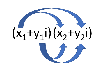
Multiplying this out gives us:
\[(x_1 + y_1 i)(x_2 + y_2 i) = x_1 x_2 + x_1 y_2 i + y_1 x_2 i + y_1 y_2 i^2\]Since $i^{2} = -1$, this simplifies to:
\[x_1 x_2 - y_1 y_2 + x_1 y_2 i + y_1 x_2 i\]The following is an example:
\[\begin{align} (3 + 2i)(4 + 3i) &= 12 + 9i + 8i + 6i^2 \\ &= 12 + 17i - 6 \\ &= 6 + 17i \end{align}\]Multiplying Two Matrices
When working with quantum states, there are three matrix by matrix multiplication operations that are commonly performed: matrix product, inner product, and tensor product (a.k.a. outer product). We look at the matrix product now and cover the inner and tensor products in later sections, as we need them.
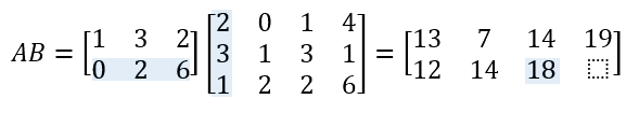
The first thing to note is that calculation of the matrix product is only valid if the number of columns in the first matrix is equal to the number of rows in the second matrix. See Figure 2.
Also notice that the row count for the result equals the row count of the first matrix, and the column count of the result, equals the column count of the second matrix.
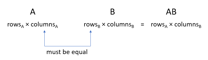
The matrix product is generally written without an operator as AB, where A and B are two matrices.
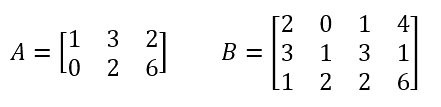
Let’s work through an example, where matrix A and B are presented below.
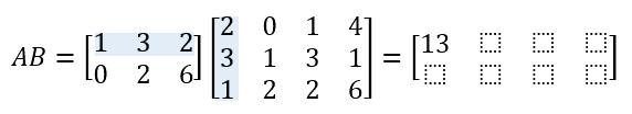
To calculate AB, we multiply each item in the first row of A by the item in the first column of B with same index, and sum the products. The result is 1×2 + 3×3 + 2×1 = 13. The value 13 is placed into the first cell of the result matrix.
We then stay on the first row of A, but we shift to the next column of B; repeating the process until we get to the end of the columns in B.
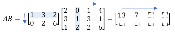
We then shift down to the second row of A, and back to the first column in B. After we complete the last row in A, we’re done.
Identifying an Element in a Matrix
By convention, a matrix is often given a capital letter as an identifier. An element within the matrix is specified using the name of the matrix in lowercase, with its row then column (in that order) shown as subscript. See the following example:
\[A = \begin{bmatrix} a_{00} & a_{01} \\ a_{10} & a_{11} \end{bmatrix}\]Multiplying a Matrix by a Scalar
The process of multiplying a matrix by a scalar is a simple one: multiply every item in the matrix by the scalar.
If A is the matrix:
\[A = \begin{bmatrix} a_{00} & a_{01} & a_{02} \\ a_{10} & a_{11} & a_{12} \\ a_{20} & a_{21} & a_{22} \end{bmatrix}\]Then multiplying the matrix by a scalar produces:
\[\lambda A = \begin{bmatrix} \lambda a_{00} & \lambda a_{01} & \lambda a_{02} \\ \lambda a_{10} & \lambda a_{11} & \lambda a_{12} \\ \lambda a_{20} & \lambda a_{21} & \lambda a_{22} \end{bmatrix}\]For example, if the scalar multiplier is 2 and A’s values are:
\[A = \begin{bmatrix} 1 & 3 \\ 5 & 2 \end{bmatrix}, \quad \lambda = 2\]Then the result is as follows:
\[\lambda A = 2\begin{bmatrix}1 & 3 \\ 5 & 2\end{bmatrix} = \begin{bmatrix}2 & 6 \\ 10 & 4\end{bmatrix}\]If the scalar is a complex number and/or the matrix contains complex numbers, the procedure does not change. You calculate the products using the rules of complex number multiplication, which we looked at earlier.
Okay, so we’ve gone over some basic math operations that you need to know to follow along. Let’s move on to something more fun.
Describing Quantum State with Dirac Notation
Dirac notation (also known as bra-ket notation) is everywhere in quantum theory. It’s used to describe quantum states. You can think of it as matrix shorthand.
A single qubit with the zero basis state can be written as a ket, like so:
\[\vert 0 \rangle\]This reads as “ket zero.”
Conversely, a qubit with a one basis state, can be written as:
\[\vert 1 \rangle\]NOTE: In some texts, |0〉 and |1〉 are presented as |↑〉 (spin-up) and |↓〉 (spin-down), respectively. When you visualize a qubit on a three dimensional sphere, |0〉 is up at the north pole and |1〉 is down at the south pole. I use |0〉 and |1〉 exclusively in this series.
Recall that |0〉 represents the column vector [1, 0]T, and 1 represent [0, 1]T.
In Dirac notation, the values within the ket—between the vertical line character ‘|’ and the angled bracket ‘〉’—are tensor products.
The symbol ‘⊗’ is used to denote the tensor product of two matrices. It is calculated by multiplying each item in the first matrix by all items in the second matrix, as illustrated:
\[\begin{alignedat}{2} \begin{bmatrix} a_{1} \\ a_{2} \end{bmatrix} \otimes \begin{bmatrix} b_{1} \\ b_{2} \end{bmatrix} &\!=\! \begin{bmatrix} a_{1}\begin{bmatrix} b_{1} \\ b_{2} \end{bmatrix} \\ a_{2}\begin{bmatrix} b_{1} \\ b_{2} \end{bmatrix} \end{bmatrix} &\!=\! \begin{bmatrix} a_{1} b_{1} \\ a_{1} b_{2} \\ a_{2} b_{1} \\ a_{2} b_{2} \end{bmatrix} \end{alignedat}\]Tensor products are condensed within Dirac notation, like so:
\[\vert 0 \rangle \otimes \vert 1 \rangle = \vert 01 \rangle\]For qubits, the Dirac notation lends itself beautifully to a binary representation. Notice below how entries in the matrix correspond to the binary, and in particular how the first entry in the matrix corresponds to 0 and not 1.
\[\vert 010 \rangle = \begin{bmatrix}0\\0\\1\\0\\0\\0\\0\\0\end{bmatrix} \;\;\longleftrightarrow\;\; \begin{array}{c c c} \text{Binary} & & \text{Decimal} \\ 000 & & 0 \\ 001 & & 1 \\ \color{red}{010} & & \color{red}{2} \\ 011 & & 3 \\ 100 & & 4 \\ 101 & & 5 \\ 110 & & 6 \\ 111 & & 7 \end{array}\]NOTE: In some texts, the leading 0’s within a ket are omitted and replaced with a subscript indicating the length. So that |0010⟩ becomes |104⟩. I don’t use that notation in this series, but you may see it elsewhere.
You can now see how |1⟩ ⊗ |0⟩ are combined by calculating the tensor product of the matrices, like so:
\[\vert 0 \rangle \otimes \vert 1 \rangle = \begin{bmatrix}1 \\ 0\end{bmatrix} \otimes \begin{bmatrix}0 \\ 1\end{bmatrix} = \begin{bmatrix}0 \\ 1 \\ 0 \\ 0\end{bmatrix} = \vert 01 \rangle\]In a quantum circuit, the inputs of the circuit are combined as tensor products. We explore this later in the series.
If the Dirac notation points to the left rather than the right, as in: 〉0|, this is called a bra. Together they form a bra-ket.
Deriving a Bra from a Ket (and Vice Versa)
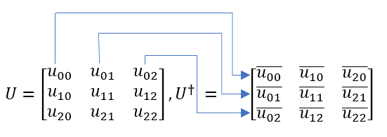
The bra is the conjugate transpose of the ket. The conjugate transpose is also known as the adjoint matrix, and yet another name is the Hermitian transpose.
To obtain the conjugate transpose, the matrix is rotated and each entry is complex conjugated. For a single column matrix, it just means we turn it horizontally and then take the complex conjugate of each entry. See Figure 3.
The complex conjugate simply means changing the sign of the imaginary part.
For example, if $z = 2 + 3i$, then the complex conjugate is $\overline{z} = 2 - 3i$.
Why Complex Numbers?
You may wonder why quantum theory relies so heavily on complex numbers. As Yanofsky and Mannucci point out [1], if you add two positive real numbers, the result will always increase. That is not the case with complex numbers. You can add two complex numbers and produce a smaller result. In fact, they may even cancel each other out. This is referred to as interference, and it is sometimes employed deliberately to eliminate unwanted states in quantum algorithms.
In the following examples we use the variables a and b, such that a,b ∈ Cd. In other words, a and b denote single column matrices of complex numbers with the number of rows equal to d. Most of the time when we are working with qubits, so the dimension count is 2.
In the following examples, we use the variables $a$ and $b$, such that $a, b \in \mathbb{C}^{d}$. In other words, $a$ and $b$ denote single-column matrices of complex numbers with the number of rows equal to $d$. Most of the time when we are working with qubits, the dimension count is 2.
The following illustrates obtaining a bra from a ket:
\[\langle a \rvert = \lvert a \rangle^{\dagger} = \begin{bmatrix}\overline{a}_{1} \\ \overline{a}_{2} \\ \vdots \\ \overline{a}_{d}\end{bmatrix}^{\mathsf{T}} = \begin{bmatrix}\overline{a}_{1} & \overline{a}_{2} & \cdots & \overline{a}_{d}\end{bmatrix}\]This process is reversible. To obtain a ket from a bra, do the same thing again: calculate the conjugate transpose.
When combined, a bra-ket ⟨b|a⟩ represents the inner product of b and a. It’s sometimes written as ⟨b,a⟩. The inner product is the sum of the products of corresponding items. This results in a complex scalar value (with or without an imaginary part). Scalar means that it’s not a vector; it’s a magnitude without direction.
\[\langle b \vert a \rangle = b \cdot a = a_{1} b_{1} + a_{2} b_{2} + \cdots + a_{d} b_{d}\]All quantum states are normalized. That is ⟨a|a⟩ = 1. This has important implications for the probability of states. We return to it in a later section.
We’ve seen that quantum theory relies on complex numbers and vectors to describe quantum states. This algebraic structure is termed a complex vector space and is also known as Hilbert Space.
Another combination of the Dirac notation, which I include for completeness, is the ket-bra. It’s written like this |a⟩⟨b| or sometimes |aXb|. A ket-bra is the tensor (or outer) product and is represented by a d × d matrix:
\[\lvert a \rangle \langle b \rvert = \begin{bmatrix} a_{1} b_{1} & a_{1} b_{2} & \cdots & a_{1} b_{d} \\ a_{2} b_{1} & a_{2} b_{2} & \cdots & a_{2} b_{d} \\ \vdots & \vdots & \ddots & \vdots \\ a_{d} b_{1} & a_{d} b_{2} & \cdots & a_{d} b_{d} \end{bmatrix}\]TIP: In quantum theory, it’s common to see the Greek characters φ (phi) and ψ (psi) used as variable names in bras and kets. For example, you often see a quantum state expressed as $\vert \psi \rangle = \dots$. Don’t be put off by the Greek characters, foreign notation, and seemingly complex algebra. It all appears far more complex than it actually is.
Exploring Quantum Superposition
We learned in an earlier section that when you measure a qubit, its quantum state collapses to either 0 or 1. To which value it collapses depends on the way the qubit has been configured. You can change the probability of a qubit collapsing to a particular value. By doing so, you place the qubit into a superposition.
Now, for a qubit that is in a pure basis state, either |0⟩ or |1⟩, the result is predetermined. It has a 100% chance of collapsing to its respective value. In other words, if you measure a qubit that was placed in the |0⟩ state, for example, you always get 0 because the probability of collapsing to 0, is 1; and the probability of collapsing to 1, is 0.
But, if you employ a certain quantum gate in your quantum circuit, you can split the probability of the qubit collapsing to 0 or 1, to a 50/50 chance either way. In which case, it is said to be in a superposition of both states.
When a qubit is in a superposition, its value is undetermined until it’s measured. In this state, it is neither 0 nor 1 in the classical sense, but a superposition of both possibilities.
This is such an unusual phenomenon, physicists have been unable to explain it using classical physics. Yet, it has been widely observed experimentally. Remember the double slit experiment? A photon seemingly goes everywhere, interfering with itself, before landing on a spot. So to does our qubit exist in all observable states until it is measured.
Disambiguating the Term “State” When one or more qubits make up a quantum system, this system has an overall quantum state at any one time. However, the system also has a set of distinct states that it may collapse to when measured. We’ll call these states: observable states.
The quantum state of one or more qubits can be described using Dirac notation and simple algebra. Observable states and associated probabilities comprise the qubit’s superposition.
A single qubit can be described by a linear combination of |0〉 and |1〉, such that:
\[\vert \Psi \rangle = \alpha \vert 0 \rangle + \beta \vert 1 \rangle\]The coefficients $\alpha$ (alpha) and $\beta$ (beta) are known as complex amplitudes or probability amplitudes. As Yanofsky and Mannucci point out [1], the name amplitude comes from the fact that a quantum state is a wave, and a wave is characterised by its amplitudes.
NOTE: Probability amplitudes are not measurable. When a qubit is measured it collapses to one of its observable states. We can manipulate the probability amplitudes, but not observe their values directly.
Calculating the Probability of Observable States
To calculate the probability of qubit collapsing to a particular state, we take the square of the modulus of its coefficient. This is known as the Born rule.
So, for the $\vert \psi \rangle$ example shown above, the probability of $\vert 0 \rangle$ is $\lvert \alpha \rvert^{2}$.
The modulus of a complex number is calculated like so:
\[\lvert x + i y \rvert = \sqrt{x^{2} + y^{2}}\]To calculate the probability we square that number. All together this can be written succinctly as shown:
\[P(x_i) = \lvert \langle x_i \vert \psi \rangle \rvert^{2}\]This is saying that to calculate the probability of the observable state $x_i$ (which is either 0 or 1 for a qubit), you square the modulus of the dot product. In other words, you project the state you are interested in onto the superposition.
Don’t worry if the algebra doesn’t make sense yet. Next we look at an example, and then we further illustrate it using matrices.
Say our qubit superposition is given by the following:
\[\vert \psi \rangle = \frac{1}{\sqrt{3}} \vert 0 \rangle + \sqrt{\frac{2}{3}} \vert 1 \rangle\]Then the probability of collapsing to 0 is given by:
\[P(0) = \lvert \langle 0 \vert \left( \frac{1}{\sqrt{3}} \vert 0 \rangle + \sqrt{\frac{2}{3}} \vert 1 \rangle \right) \rvert^{2} = \left\lvert \frac{1}{\sqrt{3}} \langle 0 \vert 0 \rangle + \sqrt{\frac{2}{3}} \langle 0 \vert 1 \rangle \right\rvert^{2}\]Now, we can reduce ⟨0|0⟩ to 1 by calculating the dot product, as shown:
\[\langle 0 \vert 0 \rangle = \begin{bmatrix}1 \\ 0\end{bmatrix} \cdot \begin{bmatrix}1 \\ 0\end{bmatrix} = 1 \times 1 + 0 \times 0 = 1\]and because ⟨0| and |1〉 are orthogonal, there inner product is 0, as shown:
\[\langle 0 \vert 1 \rangle = \begin{bmatrix}1 \\ 0\end{bmatrix} \cdot \begin{bmatrix}0 \\ 1\end{bmatrix} = 1 \times 0 + 0 \times 1 = 0\]So, if we replace those brakets in our probability formula, we see that:
\[P(0) = \left\lvert \frac{1}{\sqrt{3}} \times 1 + \sqrt{\frac{2}{3}} \times 0 \right\rvert^{2} = \frac{1}{3}\]Alternatively, we can look at the same problem, but substitute matrices for our states and calculate the probability that way.
\[P(0) = \left\lvert \begin{bmatrix}1 \\ 0\end{bmatrix} \cdot \left( \frac{1}{\sqrt{3}} \begin{bmatrix}1 \\ 0\end{bmatrix} + \sqrt{\frac{2}{3}} \begin{bmatrix}0 \\ 1\end{bmatrix} \right) \right\rvert^{2} = \left\lvert \begin{bmatrix}1 \\ 0\end{bmatrix} \cdot \begin{bmatrix} \frac{1}{\sqrt{3}} \\ \sqrt{\frac{2}{3}} \end{bmatrix} \right\rvert^{2} = \left\lvert \frac{1}{\sqrt{3}} \right\rvert^{2} = \frac{1}{3}\]Hopefully the Dirac notation version makes a bit more sense now.
Leveraging the Probability Distribution of Quantum States
We know that the sum of the probabilities in a probability distribution is always $1$. We also learned earlier that all quantum states are normalised, i.e., $\langle a \vert a \rangle = 1$. For orthonormal bases, such as $[0, 1]^{\mathsf{T}}$ and $[1, 0]^{\mathsf{T}}$, the observable states form a probability distribution. If you sum the probabilities of all observable states, they come to $1$, as described by the formula:
\[\sum_{i} P(x_i) = 1\]Therefore, we can calculate the probability of the qubit collapsing to 1, by calculating the complement of P(0), like so:
\[P(1) = 1 - P(0) = \frac{2}{3}\]Creating Multi-Qubit States
So far we’ve looked at the quantum states of single qubits. We can, of course, create quantum states with multiple qubits. These are known as multi-partite quantum states.
To do so, we combine states using tensor products. For example, if qubit A is in the state $\vert \psi \rangle_{A} = \vert 0 \rangle$ and qubit B is in the state $\vert \psi \rangle_{B} = \vert 1 \rangle$, then the total state is given by:
\[\vert \psi \rangle_{AB} = \vert 0 \rangle_{A} \otimes \vert 1 \rangle_{B} = \vert 01 \rangle_{AB}\]In this case, we can measure the state of qubit A without collapsing the state of qubit B. The individual states are said to be uncorrelated.
We can, however, place qubits into a state, where measuring one affects another. This is known as entanglement.
Entangling Qubits
For instance, take a well known state (one of the Bell states, which we discuss later), this state describes two qubits in superposition:
\[\vert \phi \rangle = \frac{\vert 00 \rangle + \vert 11 \rangle}{\sqrt{2}}\]The state of the qubits when measured will have a 50% chance of being either 00 or 11.
If we were to measure just one of the qubits, it would cause the other’s state to immediately collapse to the same value. The qubits are said to be entangled. Even if the entangled qubits are far away from each other, possibly light years. This is what Einstein described as “spooky action at a distance.”
Determining if Qubits are Entangled
When we look at the mathematics governing entanglement, we can use the matrix representation to tell us if the qubits are entangled.
As Yanofsky and Mannucci point out [1], a vector that can be written as the tensor product of two vectors is called separable.
In contrast, if the tensor product state of two qubits cannot be factored, they are said to be entangled. This is pointed out in Andrew Helwer’s introductory video on quantum computing.
For example, if we take the state |01〉, and forget for a moment that we know what the tensor product representation is already.
\[\vert 01 \rangle = \begin{bmatrix}0 \\ 1 \\ 0 \\ 0\end{bmatrix} = \begin{bmatrix}a \\ b\end{bmatrix} \otimes \begin{bmatrix}c \\ d\end{bmatrix}\]We can see that ac = 0, ad = 1, bc = 0, and bd = 0.

If we solve for a, b, c, and d; we get a = 1, b = 0, c = 0, and d = 1. We can factor it, therefore we know |01〉 is separable and not entangled.
\[\vert 01 \rangle = \begin{bmatrix}0 \\ 1 \\ 0 \\ 0\end{bmatrix} = \begin{bmatrix}1 \\ 0\end{bmatrix} \otimes \begin{bmatrix}0 \\ 1\end{bmatrix}\]In contrast, if we look at the |φ+〉 state, it is a two qubits state in equal superposition. The matrix representation is calculated below:
\[\frac{\vert 00 \rangle + \vert 11 \rangle}{\sqrt{2}} = \frac{1}{\sqrt{2}}\left(\begin{bmatrix}1 \\ 0\end{bmatrix} \otimes \begin{bmatrix}1 \\ 0\end{bmatrix}\right) + \frac{1}{\sqrt{2}}\left(\begin{bmatrix}0 \\ 1\end{bmatrix} \otimes \begin{bmatrix}0 \\ 1\end{bmatrix}\right) = \frac{1}{\sqrt{2}}\begin{bmatrix}1 \\ 0 \\ 0 \\ 0\end{bmatrix} + \frac{1}{\sqrt{2}}\begin{bmatrix}0 \\ 0 \\ 0 \\ 1\end{bmatrix} = \begin{bmatrix}\frac{1}{\sqrt{2}} \\ 0 \\ 0 \\ \frac{1}{\sqrt{2}}\end{bmatrix}\]In this case, the matrix is not factorable. We have $ac = \tfrac{1}{\sqrt{2}}$, $ad = 0$, $bc = 0$, and $bd = \tfrac{1}{\sqrt{2}}$. There is no solution for $a$, $b$, $c$, and $d$. Therefore, the matrix is not separable and the qubits are entangled. In fact, because of the equal probability of the two states $\vert 00 \rangle$ and $\vert 11 \rangle$, the Bell state is said to be maximally entangled. They are as entangled as you can get.
But, how do we create a Bell state? We explore that in Part 2 of the series. Next, we look at visualizing single qubit states.
To recap, as quantum engineers, we have the opportunity to manipulate the probabilities using quantum gates in our quantum circuits. We can also combine qubits in such a way that they correlate with one another. We can even leverage quantum entanglement to instantly affect the shared state of multiple qubits, even if the qubits are far away from one another.
Visualizing a Qubit on the Bloch Sphere
Many operations on single qubits can be neatly visualized on a 3 dimensional unit sphere, known as the Bloch sphere. See figure 4.
A qubit can be represented as a line of length 1 from the center of the sphere to the sphere’s surface.
At the north pole sits basis state |0⟩; at the south, |1⟩.
Before collapsing into a basis state, a qubit’s superposition may be located anywhere on the Bloch sphere. You can think of θ (theta) as latitude and φ (phi) as longitude. As we move vertically, north or south, the latitude changes (θ), and as we move horizontally the longitude (φ) changes.
While the latitude affects the probability of the qubit collapsing to a particular basis state, the longitude does not. The longitude is referred to as the qubit’s phase.

We saw earlier that a qubit’s superposition can be written:
\[\vert \psi \rangle = \alpha \vert 0 \rangle + \beta \vert 1 \rangle\]where α and β are its probability amplitudes, which are complex numbers.
Converting between Cartesian and Polar Representations
Recall that a complex number consists of a real part $x$ and an imaginary multiplier $y$.
\[z = x + i y\]A complex number can be represented by just $x$ and $y$. The pair $(x, y)$ is called its Cartesian representation. It can be graphed on a two dimensional Cartesian plane. Such a graph is called an Argand diagram. See figure 5.
The arg function can be used to calculate $\theta$. In this case, $\operatorname{arg}$ is equivalent to $\operatorname{atan2}$, as shown:
\[\operatorname{arg}(x + i y) = \operatorname{atan2}(y, x) = \tan^{-1}\!\left(\frac{y}{x}\right)\]Later in this section you will see how to use the $\operatorname{arg}$ function to calculate the angles $(\theta, \phi)$ on the Bloch sphere.

We can convert the Cartesian coordinates to polar representation. The polar coordinates consist of the modulus $\rho$ and the angle $\theta$. Recall that to calculate the modulus we use:
\[\rho = \lvert x + i y \rvert = \sqrt{x^{2} + y^{2}}\]To calculate the angle, we use:
\[\theta = \tan^{-1}\!\left(\frac{y}{x}\right)\]To convert back from polar to Cartesian representation, use:
\[x = \rho \cos(\theta), \quad y = \rho \sin(\theta)\]Locating the Qubit on the Bloch Sphere
Feel free to merely skim through this section. While its useful to understand how states are translated to the Bloch sphere, you can always return to this at a later stage.
The coefficients $\alpha$ and $\beta$ can be visualised on the Bloch sphere as a point corresponding to the two angles $(\theta, \phi)$.
It turns out that because $\lvert \alpha \rvert^{2} + \lvert \beta \rvert^{2} = 1$, we can calculate a qubit’s position on the Bloch sphere using the following:
\[\vert \psi \rangle = \cos\!\left(\frac{\theta}{2}\right) \vert 0 \rangle + e^{i\phi} \sin\!\left(\frac{\theta}{2}\right) \vert 1 \rangle\]where $0 \leq \theta \leq \pi$ and $0 \leq \phi \leq 2\pi$
That gives us
\[\alpha = \cos\!\left(\frac{\theta}{2}\right) \quad \text{and} \quad \beta = e^{i\phi} \sin\!\left(\frac{\theta}{2}\right).\]To find the angles, use
\[\theta = 2 \cos^{-1}(\lvert \alpha \rvert) \quad \text{and} \quad \phi = \operatorname{arg}(\beta) - \operatorname{arg}(\alpha).\]NOTE: You can also find these values via the state’s density matrix, which is calculated by its ket–bra: $\rho = \vert \psi \rangle \langle \psi \vert$. This is outside the scope of this article.
Conclusion
In this article, we explored the differences between qubits and classical bits. We looked at the computation basis for qubits. We saw how to describe quantum state using Dirac notation. We observed that qubits can be placed into superposition, and saw how to calculate the probability of observable states. We also saw how an entangled qubit can affect the quantum state of the pair. Finally we took a ride around the Block sphere, and saw how a qubit’s state can be visualized in 3 dimensions.
In the next part, we explore how quantum gates are used to build quantum circuits, which ultimately puts us on the road to materializing quantum algorithms. I hope you’ll join me.
Thanks for reading and I hope you found this article useful. If so, then I’d appreciate it if you would please rate it and/or leave feedback below.
References
The following sources were used in the preparation of this article:
-
Yanofsky, N., & Mannucci, M. (2008). Quantum Computing for Computer Scientists. Cambridge University Press.
-
Anton, H. (2000). Elementary Linear Algebra (8th ed.). Wiley.
-
Nielsen, M., & Chuang, I. (2010). Quantum Computation and Quantum Information (10th ed.). Cambridge University Press.
-
Glendinning, I. (2005). The Bloch Sphere.
https://www.vcpc.univie.ac.at/~ian/hotlist/qc/talks/bloch-sphere.pdf -
Dutta, S. (2019). If quantum gates are reversible how can they possibly perform irreversible classical AND and OR operations?
https://quantumcomputing.stackexchange.com/questions/131/if-quantum-gates-are-reversible-how-can-they-possibly-perform-irreversible-class -
Wolf, R. (n.d.). Quantum Computing: Lecture Notes.
https://homepages.cwi.nl/~rdewolf/qcnotes.pdf -
Wikipedia contributors. (2019). Quantum logic gate.
https://en.wikipedia.org/wiki/Quantum_logic_gate -
Glendinning, I. (2010). Rotations on the Bloch Sphere.
https://www.vcpc.univie.ac.at/~ian/hotlist/qc/talks/bloch-sphere-rotations.pdf -
Hui, J. (2018). What are Qubits in Quantum Computing?
https://medium.com/@jonathan_hui/qc-what-are-qubits-in-quantum-computing-cdb3cb566595
Previous Discusssion
This article was originally published on CodeProject, where reader comments available: